Welcome to Part 9 in the Fundamentals of Aircraft Design series. In the previous posts we have covered the fundamentals of flight, studied the wing, fuselage and empennage, and have been introduced to aerodynamic lift, drag and moment coefficients. Now we put it all together and run through a preliminary drag estimation of a new aircraft design.
Up to this point in the series we have used many “rules-of-thumb” or studied existing aircraft when generating a concept aircraft. Looking at and using past aircraft data provides a solid starting point in a new design but it does not confirm that we will meet the mission requirements set out for the design. It’s now time to take the next step as we begin to build a mathematical performance model, which will enable us to estimate the total drag produced by the design as a function of the chosen aircraft geometry.
Drag Estimation - Prerequisites
In order to complete this tutorial you will need to be familiar with the following concepts outlined in previous posts:
If you haven’t done so already, read through the above posts before continuing with this tutorial.
User Requirement Specification
Every new aircraft starts with a list of user requirements. It is very important to clearly define the intended purpose of the aircraft before going ahead with the initial sketches and layout. Some typical questions that should be asked before generating a new concept are:
- What is the primary mission - passenger, cargo, maritime patrol, military fighter, troop transport etc?
- What is the size and mass of the intended payload (passengers, cargo, weapons)?
- At what altitude will the aircraft predominantly operate?
- What is the intended cruise speed?
- Define the typical airports/landing strips from which the aircraft will operate.
- Does the aircraft require cabin pressurization?
- Is take-off performance or cruise speed of greater importance to fulfill the mission requirement?
- What is the approximate mass of the aircraft (EW, MTOW, payload)
With this information clearly defined you can start to generate a conceptual representation of the aircraft by following the steps outlined in the previous posts. Your conceptual representation should include such variables as maximum take-off weight, cruise speed, and a sketch of the conceptual aircraft layout. With this conceptual layout and mass estimation completed you can move onto the initial performance estimation - the drag calculation.
In this tutorial we will define the preliminary geometry of a two-seat light aircraft, go through the initial drag estimation exercise, and create a number of plots that describe how the aircraft drag varies with velocity and the amount of lift produced. This will assist us in selecting a power unit (engine and propeller - see Part 10 in this series) and ultimately calculating the maximum theoretical speed of our design.
Preliminary Design Geometry
For the purposes of this tutorial we will follow a worked example approach. Below is a sketch of a conceptual two-seat light sport aircraft (LSA) designed to cruise between 80 and 100 kts.
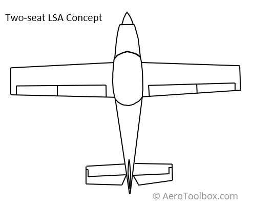
All the required geometry with which to perform the drag estimation is shown in the table below. We will work in SI (metric) units when performing our preliminary drag estimation.
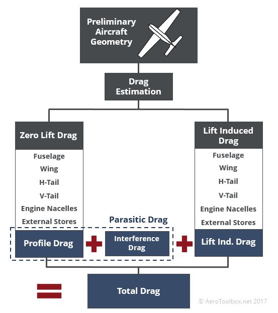
Drag Breakdown
Our aircraft consists of a number of major components which each contribute to the total drag produced: wing, fuselage, empennage (horizontal and vertical tail) and canopy. Larger aircraft could also have engine nacelles, external stores, fairings or antennae that should also be included in the drag calculation.
Broadly we split the drag contribution of each component into two distinct categories: Parasitic (zero-lift) drag and Lift Induced drag. It’s important to note here that our concept aircraft operates far away from the transonic or sonic flight regime and so drag due to the compressibility of the air (wave drag) is not a factor in this analysis.
Parasitic drag: Drag produced as a consequence of the shape and form of the body interacting with the medium through which it passes (here air).
Lift Induced drag: Drag produced as a consequence of the lift force generated by the body.
The total aircraft drag is therefore the sum of the zero-lift drag (parasitic) and the lift-induced drag.
$$ C_{D_{tot}} = C_{D_{0}} + C_{D_{i}} $$
\( C_{D_{tot}}: \) Total drag (drag coefficient)
\( C_{D_{0}}: \) Zero-lift drag coefficient
\( C_{D_{i}}: \) Lift-induced drag coefficient
Parasitic Drag
Parasitic drag is the term given to the drag component that results when an object is moved through a fluid (in our case air). There are three major components to parasitic drag: skin friction drag, pressure (form) drag, and interference drag. We’ll look at each separately, show how to calculate each component, and then add them together to arrive at a final parasitic drag term.
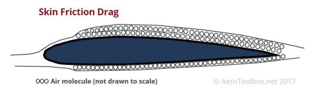
Skin Friction Drag
Skin friction drag arises from the interaction between the aircraft skin and the fluid (air) molecules that come into contact with the skin. As the aircraft flies along, air molecules come into contact with the skin and tend to stick to it. This is analogous to the way water molecules stick to your skin when swimming. Each air molecule that is stuck to the skin in turn causes adjacent molecules to stick to itself and a boundary layer of air forms around the aircraft body. This boundary layer of air molecules must be pulled through the atmosphere as the aircraft flies. It is this additional drag formed by the layer of air which is termed skin friction drag. The frictional component of drag is a function of the wetted area of the body in question which is defined as the area of skin in contact with the fluid (air).
Pressure Drag
Pressure (form) drag is the component of drag that arises as a result of the shape of the body and the effect that the shape has on the resulting local pressure distribution (in the drag direction). Different shapes will produce varying amounts of pressure drag. On the one extreme, would be a flat plate oriented normal to the direction of flow. There will exist a large pressure drop across the plate with a correspondingly large pressure drag resulting. On the other hand, a thin, streamlined, bullet-like body will produce a much smaller pressure drop and corresponding pressure drag force.
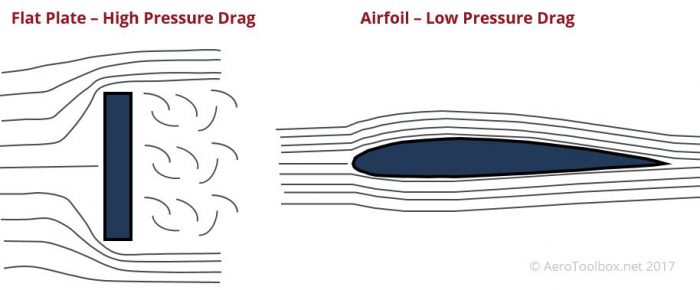
The cross-sectional area and longitudinal variation in the cross-section are two very important parameters when calculating pressure drag. A good indication of the relative magnitude of the resulting pressure drag is to consider the fineness ratio of the aerodynamic body. This is the ratio of the length of the body to its maximum diameter. Generally a fineness ratio of approximately 6 provides an optimized shape.
Interference Drag
Interference drag results from the interaction of surfaces in contact with one another. A good example is at the interface between the wing and the fuselage. The resulting drag force is greater than the individual drag values calculated for the wing and fuselage in isolation. The difference is attributed to interference.
Let's now look at the various major aircraft components that make up our fictional light sport aircraft and begin to put together our parasitic drag estimation. We follow a process known as drag 'book-keeping' where the drag contribution for each component (wing, fuselage, tail, engines etc) is first estimated and finally tallied up to arrive at a final parasitic drag estimation. The lift-induced drag component is then added to give a final drag variation with speed.
Fuselage Zero Lift (Profile) Drag
We start with the profile drag contribution of the fuselage. The following formula is an approximation to the zero-lift drag produced by the fuselage. The calculation is primarily a function of the fuselage wetted area \( \left( S_{wetF} \right) \) and the fuselage fineness ratio \( \left( \frac{l_{f}}{d_{f}} \right) \).
The skin friction coefficient and wing to fuselage interference factor can be obtained using the links to the calculators provided.
$$ C_{D_{0(fus)}} = R_{wf} \cdot C_{f(fus)} \left \{ 1+\frac{60}{ \left( \frac{l_{f}}{d_{f}} \right) ^{3}} + 0.0025 \times \left( \frac{l_{f}}{d_{f}} \right) \right \} \cdot \frac{S_{wetF}}{S_{ref}} $$
Where:
\( R_{wf}: \) Wing/fuselage interference factor (if fuselage is considered in isolation then \(R_{wf}\) = 1)
\( C_{f(fus)}: \) Turbulent flat plate skin-friction coefficient of the fuselage. Use fuselage length to determine Reynolds No.
\( l_{f}: \) Fuselage Length \( d_{f}: \) Maximum fuselage diameter (equivalent diameter can be used for non-circular cross-section).
\( S_{wetF}: \) Fuselage wetted area (fuselage surface area exposed to air)
\( S_{ref}: \) Aircraft reference wing area
If the fuselage diameter is not circular (or approximately circular) an equivalent diameter can be calculated based on the maximum fuselage cross-section.
$$ d_{f_{equiv}} = \sqrt{\frac{4}{\pi}\cdot{S}_{fus_{Max}}}$$
Where:
\( d_{f_{equiv}}: \) Fuselage equivalent diameter
\( {S}_{fus_{Max}}: \) Maximum fuselage cross-sectional area
The fuselage \( C_{D_{0(fus)}} \) value is not constant across all speeds and altitudes. The variation arises from the fact that the skin friction coefficient and the fuselage interference factor are both a function of the Reynolds number, which is in turn a function of the aircraft velocity and atmospheric conditions (density and temperature). In some cases during the conceptual design phase the value may be assumed constant if it can be shown that the variation in drag value is minimal over the range of velocities and altitudes considered.
The variation in zero-lift fuselage drag for our concept LSA is plotted below:
Wing Zero Lift Drag
Next we look at the profile drag contribution of the wing to the aircraft total. Remember that the total drag contribution of the wing consists of zero-lift and lift-induced components.
Here we are only concerned with the zero-lift component. The formula shown below is used to approximate the zero-lift wing drag. As with the fuselage, the drag is primarily a function of the applicable wetted area \( \left( S_{wetW} \right) \).
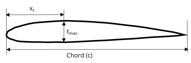
The wing's thickness-to-chord ratio \( \left( \frac{t}{c} \right) \) is also a major driver of the resulting profile drag. It follows that an increase in the thickness of the wing results in a greater impediment to the motion of air over and around the wing. In cases where the thickness-to-chord ratio varies along the span of the wing, the average value should be used in the calculation.
We introduce a number of additional terms in the equation below; namely a lifting surface correction factor, and a factor termed \( \left( L^{*} \right) \) which is an airfoil thickness location parameter.
$$ C_{D_{0(wing)}} = R_{wf} \cdot R_{LS} \cdot C_{f(wing)} \left \{ 1+ L^{*} \cdot \left( \frac{t}{c} \right) + 100 \cdot \left( \frac{t}{c} \right) ^{4} \right \} \frac{S_{wetW}}{S_{ref}}$$
Where:
\( R_{wf}: \) Wing/fuselage interference factor (if flying wing then \(R_{wf}\) = 1)
\( R_{LS}: \) Lifting surface correction factor
\( C_{f(wing)}: \) Turbulent flat plate skin-friction coefficient of the wing. Use wing chord to determine Reynolds No.
\( L^{*}: \) Airfoil thickness location parameter
\( \left( \frac{t}{c} \right): \) Airfoil thickness-to-chord ratio
\( S_{wetW}: \) Wing wetted area
\( S_{ref}: \) Aircraft reference wing area
\( \left( L^{*} \right) \) is concerned with the location of the maximum thickness of the wing. Broadly speaking, a value of 1.2 should be used for a NACA 4 or 5 Series airfoil and a value of 2.0 for NACA 6 Series and supercritical airfoils. The formal definition is shown in the image below.
Using the wing zero-lift equation we can plot the variation of wing profile drag with velocity for our concept LSA.
Horizontal and Vertical Tail
The horizontal and vertical tail are aerodynamic surfaces and as such the methods used to calculate the wing zero-lift drag hold for these surfaces too. Keep in mind that the vertical stabilizer should make use of a symmetrical airfoil profile which negates the need to include a lift-induced drag contribution unless the aircraft is in a side-slip. The horizontal tail will produce a balancing trim force at cruise which we neglect at this conceptual design phase.
The zero-lift drag contribution of the empennage on our concept LSA is plotted below.
Interference and Excrescence Drag
Up to this point we have calculated the total zero-lift drag as the sum of the individual components present on the aircraft (fuselage, wing, empennage). However this methodology does not take into account two additional sources of drag; namely Interference and Excrescence drag.
Interference Drag
Interference drag arises from the interaction of airflow between two bodies which are connected in some way. Some examples are the interface between the wing and the fuselage, or the location of engine nacelles either under the wing or on the body of the fuselage. In all cases the resulting drag is greater than the sum of the individual drag contributions. This difference is given the broad term, interference drag.
The increase in drag is attributed to the interaction between boundary layers or pressure fields which alters the resulting flow. It is very difficult to accurately determine the contribution of interference to the total drag of the aircraft unless wind tunnel tests or flow simulations have been completed. At the conceptual phase in the design it is sufficient to estimate an interference factor and add that to the total zero-lift drag value for the aircraft.
Excrescence Drag
Another form of aircraft drag that is difficult to quantify comes from the various sensors, antennae, and finishings present on an aircraft. At the conceptual stage these are all lumped under the term excrescence. Excrescence is defined as, "a distinct outgrowth on a body or plant, resulting from disease or abnormality. which nicely defines this contributor to drag. While each individually small, the sum of all these appendages to the surface of the aircraft can be really significant.
Some of the more common components adding to excrescence drag are:
- Radio antenna for communication
- GPS receiver
- VOR antenna
- UHF antenna
- ADF antenna
- Pitot Static Probe
- Rivets or screws
- Windscreen wipers
- Vortex generators
- Navigation lights
Interference & Excrescence Drag Factor
Appendages attached to the fuselage will also produce a component of interference drag. Thus the excrescence and interference drag contribution is linked. At the conceptual stage in the design process it is convenient to lump all these drag contributors together and estimate a single factor by which we multiply the previously estimated profile drag value.
A correction factor is estimated based on the category of aircraft being designed. This is certainly not an exact science but the factors shown below will be sufficiently accurate at this early stage.
| Aircraft Type | Drag Factor \( \left( K_{C} \right) \) |
|---|---|
| General Aviation | 1.20 |
| Piston (single) | 1.30 |
| Agricultural | 1.50 |
| Subsonic Jet | 1.10 |
| Supersonic Jet | 1.10 |
| Glider | 1.05 |
Our LSA concept is designed to be of modern construction (composite rather than metallic) and being a Light Sport Aircraft should have fewer external antennae than traditional certified general aviation aircraft.
As an estimate we'll make use of a factor of 1.15 to account for interference and excrescence.
Book-keeping Drag Table (Total Zero-lift Drag)
Now that we have accounted for the zero-lift drag contribution of all the major components on our conceptual aircraft we sum them together to calculate the total zero-lift drag \( C_{D_{0}} \).
The total parasitic drag term can therefore be written:
$$ C_{D_{0}} = K_{C} \times \left[ C_{D_{0(wing)}} + C_{D_{0(fus)}} + C_{D_{0(ht)}} + C_{D_{0(vt)}} \right] $$
Of course the equation above could also include engine nacelles (modelled using the fuselage equation), pylons, struts, external stores etc depending on the aircraft configuration. As mentioned above, the \( C_{D_{0}} \) value varies with speed and altitude. We have assumed that our aircraft is operating at Sea Level in a standard atmosphere but this may not be the case.
The term book-keeping drag is given to the method by which the individual contributions of drag are summed together and displayed in a table - similar to what is shown below. The drag table below is interactive and the effect of cruise speed on the \( C_{D_{0}} \) value can be seen using the drop-down menu.
| Component | ||
|---|---|---|
| Fuselage | ||
| Wing | ||
| H-tail | ||
| V-tail | ||
| Total Profile | ||
| + Interference (15%) | ||
| \(C_{D_{0(tot)}} \) |
Lift Induced Drag
As the name implies, lift-induced drag is the drag force that is formed as a by-product to the generation of lift. As it is the wing which is primarily responsible for the generation of lift, it follows that this is the major contributor. However, any body inclined at an angle of attack relative to the direction of the free-stream will produce a lifting (or downward) force; so engine nacelles, a fuselage, under-wing stores or the horizontal tail can all contribute to the total lift-induced drag.
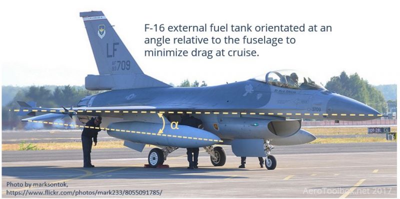
We will focus our efforts on the wing since it is primarily responsible for the generation of lift-induced drag. It is the goal of any aircraft designer to minimize the drag produced by the aircraft. Good design practice is therefore to orientate the fuselage, engine nacelles, and any underwing external stores, such that at cruise they produce no net vertical force (lift or downforce) and therefore produce a negligible lift-induced drag.
A good example of this is seen when looking at many fighter aircraft such as the F-16 pictured below. Here the external fuel tank is orientated at an angle relative to the fuselage. This is to reduce the lift-induced drag component of the external store during cruise. The F-16's optimum cruise angle much be such that the fuselage is inclined at a slight positive angle; and so if the external store was orientated at the same angle it would cause the store to produce a lifting force and consequently a lift-induced drag component.
Using our example of the concept LSA, we will only consider the wing's contribution to the lift-induced drag as it is the primary contributor.
Wing Lift Induced Drag
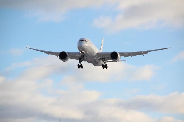
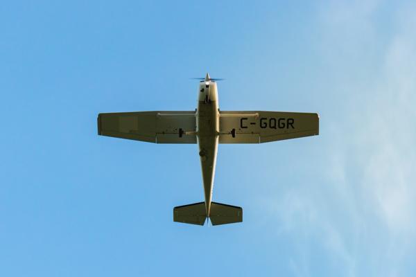
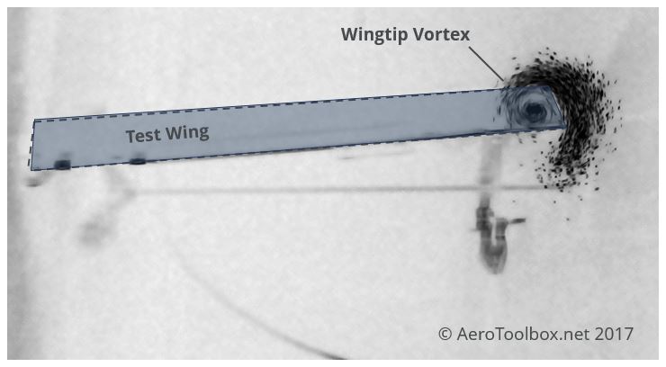
A wing produces lift as a result of the pressure gradient that exists between its upper and lower surface. The increased curvature on the upper surface results in a pressure drop relative to the lower surface. As the tip of the wing is approached, there still exists a pressure difference between the two surfaces, however there is now nothing to impede the movement of air from the lower surface to the upper. This causes the air to roll up and over the upper surface and form a wingtip vortex on the tip of each wing which propagates through the atmosphere and impedes the aircraft motion through the air (lift induced drag).
The wingtip vortex is well captured in the photograph below.
The formula used to calculate the lift-induced drag produced by a wing is a function of the square of the lift-coefficient. Induced drag therefore increases exponentially with an increase in the lift coefficient and so is most prevalent at low speed where the lift coefficient is highest.
$$ C_{di} = \frac{{C_{LW}}^2}{\pi \cdot AR \cdot e} $$
$$ C_{LW} = 1.05 \cdot C_{L} $$
Where:
\( C_{LW}: \) Lift produced by the wing (5% added to account for H-tail trim force)
\( C_{L}: \) Aircraft lift coefficient
\( AR: \) Aircraft Aspect Ratio
\( e: \) Oswald efficiency factor
The aircraft lift coefficient is a function of the aircraft mass, atmospheric conditions, and velocity.
$$ C_{L} = \frac{2 \cdot M \cdot n \cdot g}{\rho \cdot S_{ref} \cdot V^{2}} $$
Where:
\( M: \) aircraft mass
\( n: \) aircraft load factor (n = 1 for straight and level cruise)
\( g: \) acceleration due to gravity
\( \rho: \) air density (see atmospheric calculator)
\( S_{ref}: \) Aircraft reference wing area
\( V: \) aircraft velocity
A factor of 5% (1.05) is added to the wing lift coefficient as the wing must produce more lift than the mass of the aircraft due to the balancing force required to trim at the horizontal tail.
The Oswald efficiency factor is a measure of the spanwise efficiency of the wing. Refer to the post on wing structural design to see an illustration of how the lift along the span of a wing varies as one moves from the root to the tip. An aircraft with an elliptical wing, such as a Spitfire, produces the ideal spanwise lift distribution \( \left( e = 1 \right) \). Most general aviation wings are rectangular or tapered and a good approximation to the Oswald factor is between 0.75 and 0.85. The table below may be used to approximate the factor.
| Aircraft Type | Oswald Factor (e) |
|---|---|
| General Aviation | 0.70 - 0.80 |
| Twin Turboprop | 0.75 - 0.80 |
| Agricultural | 0.65 - 0.70 |
| Subsonic Jet | 0.75 - 0.85 |
| Supersonic Jet | 0.60 - 0.80 |
| Glider | 0.80 - 0.90 |
The Oswald Efficiency factor of our concept LSA is estimated to be equal to 0.80.
Now that we have covered the basics of drag estimation of lifting surfaces (wing, horizontal tail, vertical tail) and streamlined bodies (fuselage, engine nacelle, external stores) we can put all of the various components together to plot the variation of the total aircraft drag with velocity. We will also investigate a drag polar plot which can be used to describe the state of the aircraft at any moment in time.
Putting it all together
Drag Variation with Velocity
The final aircraft drag calculation is a matter of summing the parasitic and induced drag values together to arrive at a final drag coefficient which represents the total drag acting on the aircraft for a given velocity and atmospheric condition.
Drag Coefficient
Remember that the aircraft drag coefficient is not constant but will vary with atmospheric condition, velocity, and the lift coefficient. Therefore the best way to depict the drag coefficient is to do so across the aircraft's intended speed range by either building a spreadsheet or alternatively writing a computer script that will repeat the calculation across the desired speed range and atmospheric conditions.
In the case of this conceptual LSA (light sport aircraft) a script has been written that calculates the drag coefficient between 60 kts and 160 kts (the intended speed range of the aircraft). It has been assumed that the aircraft is flying at Sea Level in a Standard Atmosphere (atmospheric calculator). The variation in drag coefficient is plotted below.
You will notice that the parasitic drag is nearly constant through the speed range considered here. In the early stages of design it may be permissible to assume this value is a constant provided the aircraft is operating far away from the transonic region where the compressibility of air is not a factor (see the post on drag divergence for further reading).
At low speeds, the drag coefficient is largely driven by the induced drag component which is due to the high lift coefficient required to fly near the stall. As the speed is increased, the lift coefficient reduces and the parasitic drag effects begin to dominate. At 160 kts the aircraft drag coefficient is almost entirely a function of the parasitic drag term.
Total Drag Force
We show above that the drag coefficient reduces with velocity but this does not imply that the drag reduces with velocity. In fact the total drag is a function of the dynamic pressure which is a function of the square of the velocity.
Recall the equation used to define the drag coefficient: $$ C_{D} = \frac{D_{tot}}{q_{\infty} \cdot S_{ref}} = \frac{D_{tot}}{\frac{1}{2} \cdot \rho \cdot V_{\infty}^2 \cdot S_{ref}} $$ Rearranging and solving for Total Drag: $$ D_{tot} = q_{\infty} \cdot S_{ref} \cdot C_{D} $$
Where:
\( q_{\infty}: \) Dynamic Pressure ( \( \frac{1}{2} \cdot \rho \cdot V_{\infty}^2 \) )
These definitions allows one to plot the variation with drag (measured here in Newtons) with the variation in airspeed (knots). The relationship is parabolic in nature due to the increase in drag with the square of the velocity.
The resulting drag curve is often called a drag bucket as the plot resembles a bucket with high drag at speed extremes (low and high) and a minimum drag value at some intermediate speed. This is the bottom of the so called bucket and is the speed at which it is most efficient to fly (requires the least amount of thrust to overcome drag). Our conceptual aircraft produces a drag minimum at approximately 80 kts which is the low end of our envisioned cruise speed.
The piechart shown below provides a further breakdown of the total drag into its various components. You can use the drop-down menu below to see how the breakdown varies with speed. Induced drag dominates at low speed and parasitic drag is the driver at high speed.
The Drag Polar
A final means to represent the variation in drag is to plot the variation in drag coefficient with the corresponding aircraft lift coefficient. This plot is known as a drag polar and provides a snapshot of the aircraft's performance for the entire flight envelope (at a given atmospheric condition and altitude). Dividing the lift coefficient by the drag coefficient results in a value know as the lift-to-drag ratio or the aerodynamic efficiency. The point at which this is a maximum yields the most efficient point at which to fly. Here the ratio of lift-to-drag is at a maximum.
It should come as no surprise that the point where the lift-to-drag ratio is a maximum corresponds to the lowest point in the drag bucket plot (lowest drag). The lift coefficient corresponding to this point then forms the basis of the airfoil profile selection as a profile should be selected that produces minimum drag at the required lift coefficient.
This brings us to the end of this tutorial on how to develop and plot the drag breakdown of an aircraft. Using the knowledge gained here, you should be able to produce your own drag estimation on any subsonic aircraft operating away from the transonic region.
The final tutorial in this Fundamentals of Aircraft Design Series looks at how to overlay a thrust variation with speed onto the drag curve to calculate the aircraft's theoretical maximum speed.
Thanks for reading this tutorial on generating a drag curve and polar. If you enjoyed reading this please get the word out and share this post on your favorite social network or recommend this site to your friends and colleagues!