Introduction
In the previous post we introduced the four fundamental forces acting on an aircraft during flight: Lift, Drag, Thrust and Weight and examined how they interact with one-another. We are now going to look more closely at the two aerodynamic forces Lift and Drag. We will look at the relationship between the two forces, study how they interact with one another, and learn how to non-dimensionalize the resulting forces.
Two of the four fundamental forces acting on an aircraft during flight come about as a result of the aerodynamic loading on the body as it flies through the air. If you have read the previous post you will understand that lift must be produced by the airplane wing in order to act as a counter-force to the total flying weight, and that as a natural consequence to the motion of the aircraft through the air, a drag force that opposes this motion is also present. In this post we will examine how and why aerodynamic forces are generated as the airplane moves through the air, and introduce a method to non-dimensionalize the forces such that aircraft of various shapes and sizes can be directly compared to one-another.
We are going to specifically focus on the wing for the rest of this tutorial but the concept behind aerodynamic loading can just as easily be extended to any other component of the aircraft such as the fuselage, an engine cowling or even a canopy.
Pressure and Shear Loading
If you have ever stuck your hand out of a moving vehicle and felt the force of the air pushing on your hand you should intuitively have a pretty good idea of the concept of lift and drag. In this case the lift force tends to push your hand upward while the drag force pushes your hand backward. Here the force being exerted on your hand is being generated by two force distributions acting on your hand: a pressure distribution and a shear distribution.
Exactly the same thing happens when we consider an airfoil subjected to a flow of air over its surface: a pressure and shear distribution are present acting over the entire airfoil surface.
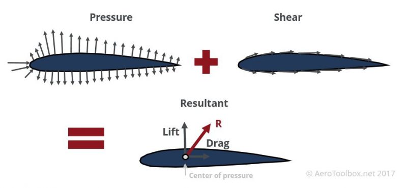
The pressure distribution acts locally perpendicular (normal) to the airfoil surface.
The shear distribution acts locally parallel to the airfoil surface.
Taking the local pressure contribution at each point along the surface and adding each contribution together (integration) results in a net pressure force acting on the airfoil. Similarly, adding the shear contribution along the airfoil surface results in a net shear force.
The resultant aerodynamic force acting on the airfoil is therefore the sum of the pressure and shear contributions.
It is important to remember that the above result is true irrespective of the shape of the surface in question; the net aerodynamic force acting on any body in a free stream of air will always be the sum of the pressure and shear distributions acting along the body.
Center of Pressure
The net vertical force is termed the lifting force and the net horizontal force is termed the drag force. The net lift and drag force acts at the center of pressure of the airfoil. However, the center of pressure is not a fixed point and will vary as the angle of attack of the airfoil is varied.
Quarter Chord
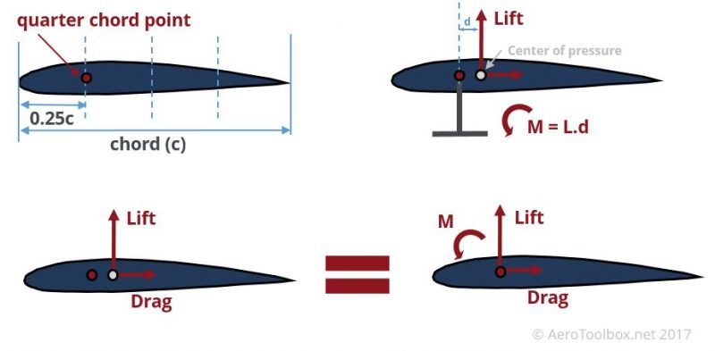
The center of pressure is therefore not a convenient location about which to specify the resultant forces acting on the airfoil as it is not fixed. A common convention is to use a point specified at the airfoil quarter chord. This is a point located one quarter of the way along the chord from the leading edge. Moving the resultant lift and drag force from the center of pressure to the quarter chord requires that a moment be added to achieve a force balance. Thus a pitching moment equal to the lift force multiplied by the moment arm between the quarter chord and the center of pressure is added to achieve static equilibrium (Here we have neglected the component of the shear force that would contribute to the total pitching moment as it is negligibly small relative to the lift component).
We can therefore specify the resulting aerodynamic force on the airfoil as a lift and drag force acting at the quarter chord plus a balancing pitching moment.
Non-dimensional Coefficients
We have shown above that the aerodynamic properties of any body can be represented by resolving the resulting force into its normal (lift) and parallel (drag) components. We have also illustrated how it is often convenient to represent the resulting force on the body in terms of its force components and a moment about a fixed arbitrary point (the quarter chord in our example).
How though do we compare multiple aerodynamic surfaces to one another as every surface will produce a particular net force based on parameters such as free-stream velocity, density of the medium, the wetted area of the body, the angle of attack of the body and the compressibility of the medium flowing over the body?
The answer lies in a clever use of mathematics, performing an exercise where the various forces are non-dimensionalized.
Each aerodynamic force is a function of the following parameters:
$$ F = fn(V_{\infty}, \rho, \alpha, \mu, a_{\infty}) $$ Where: \( V_{\infty} \) = free-stream velocity \( \rho \) = density of the medium \( \alpha \) = angle of attack \( \mu \) = viscosity of the medium \( a_{\infty} \) = Free stream sonic speed
We can therefore non-dimensionalize the forces and moment in the following way:
$$ C_{L} = \frac{L}{q_{\infty}S} $$
$$ C_{D} = \frac{D}{q_{\infty}S} $$
$$ C_{M} = \frac{M}{q_{\infty}Sc} $$
Where:
\( L \) = Lift Force
\( D \) = Drag Force
\( M \) = Moment
\( S \) = Reference Area (usually Wing Area)
\( c \) = Reference Wing Chord
\( q_{\infty} \) = Dynamic pressure (\( \frac{1}{2} \rho V_{\infty}^2) \)
These non-dimensional representations of the lift, drag and pitching moment allow one to compare two aerodynamic bodies of different size, shape, and orientation to one another having normalised the result to account for the variation in the force produced by the size of the body and the conditions of flow.
Flow Similarity
The non-dimensional coefficients listed above don’t fully describe force components and moments as a number of parameters are not included in the definition above. We introduce two additional flow similarity parameters Reynolds Number and Mach Number to fully describe the flow.
$$Re = \frac{Inertial Forces}{Viscous Forces} = \frac{\rho V L}{\mu} = \frac{V L}{\nu}$$ $$ M_{\infty} = \frac{V_{\infty}}{a_{\infty}} $$
Where:
\( L \) = Characteristic length of the body (often wing chord or fuselage length in aeronautical design)
\( \mu \) = Dynamic viscosity of the fluid
\( \nu \) = Kinematic viscosity of the fluid \( (\nu = \frac{\mu}{\rho}) \)
\( M_{\infty} \) = Mach number
\( V_{\infty} \) = free-stream velocity
\( a_{\infty} \) = Free stream sonic speed
It is common practice to generate a set of aerodynamic data across a range of angles of attack to understand how the aircraft or vehicle behaves as its attitude is varied. This allows engineers to ensure that the aircraft behaves safely and predictably through its entire design envelope. This data is most often gathered by performing a set of wind tunnel tests, using a model of the aircraft or vehicle being designed.
However, it would be prohibitively expensive to attempt to complete tunnel tests of a full-scale model as the size of the tunnel and the amount of energy required to reach the flying speeds of a typical aircraft would be astronomical. Instead using the equations defined above, the engineer can model a dynamically similar flow on a scale model by ensuring that the Reynolds Number and Mach Number of the real aircraft and the model match one another.
This is a very powerful result as the actual response of a full scale airplane can be modeled at scale in a smaller tunnel by ensuring flow similarity.
It is often difficult to achieve both a matching Reynolds Number and Mach number on a single test; but often the conditions can be modeled such that a good approximation to the actual flight test data can be reached.
Coefficient Variation with Angle of Attack
For this discussion we will limit ourselves to discussing a wing cross-section as the relationship between lift, drag and angle of attack of an airfoil profile is well established. A similar analysis could be conducted on any aerodynamic body such as a fuselage, canopy, external fuel tank or fairing although good aerodynamic data on more obscure shapes is difficult to find. The best way to obtain high-quality aerodynamic data on an uncommon body would be to perform a series of wind tunnel tests in order to generate the required data oneself. A Computational Fluid Dynamics (CFD) simulation can also be run to generate aerodynamic data but one must be conscious of the limitations of the simulation before using the data generated. CFD simulations can be very useful and provide a lower cost approach to gathering aerodynamic data but the solver must be thoroughly validated and bench-marked before being used.
The angle between a reference line on a body and the vector representing the relative motion between the body and the fluid through which it is moving is termed the angle of attack. This is demonstrated on an airfoil profile below:
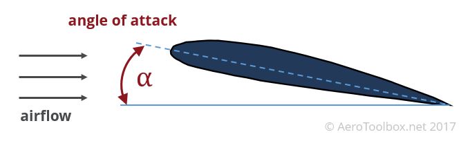
It is intuitive that the lift and drag force produced by the wing will vary with the angle of attack, as the local pressure and shear distribution around the wing will change as the wing is rotated in the freestream.
Non-dimensionalizing the lift and drag values and plotting this across a range of angles of attack means that a number of airfoil profiles or configurations may be compared such that the most suitable design is selected. Most of the time the most suitable configuration will be the one that minimizes drag as it is easier to produce sufficient lift from a wing than to produce a minimum amount of drag.
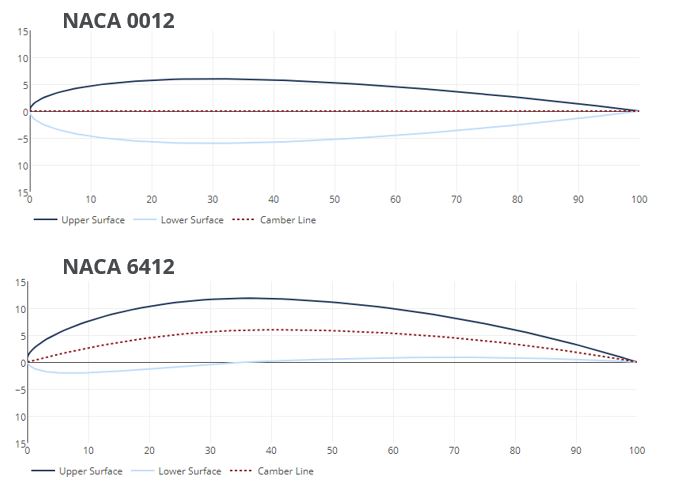
NACA Four Series Airfoil Example
The variation of lift and drag coefficient with angle of attack is shown below for a NACA 0012 and NACA 6412 profile (you can plot the profiles yourself using the NACA 4 Series Plotting Tool). The aerodynamic data was compiled using a tool called xFoil for a Reynolds Number equal to 1 million.
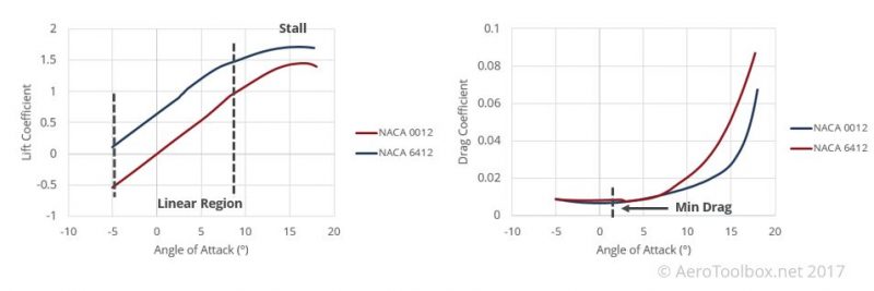
Increasing the angle of attack of the airfoil produces a corresponding increase in the lift coefficient up to a point (stall) before the lift coefficient begins to decrease once again.
There are three distinct regions on a graph of lift coefficient plotted against angle of attack.
- Linear region: where the lift coefficient increases linearly with the angle of attack
- Non-linear region: (pre-stall) here an increased angle of attack still results in an increase in the lift coefficient but this is not linear as flow separation effects begin to appear.
- Post stall region: here the angle of attack is past the critical stall point (maximum lift coefficient), and while the airfoil is still generating lift, the drag has increased exponentially. One should avoid flying an aircraft past the point of stall. A stable aircraft will tend to drop its nose post stall, thereby reducing the angle of attack back into the linear region.
The plot of drag vs angle of attack tends to form a bucket shape with a local minimum (minimum drag) at a particular angle of attack for a particular airfoil. A well designed airfoil should allow one to fly through a range of low angles of attack (linear lift region) without encountering too large a drag penalty. The total drag is a function of both the shape of the airfoil (profile drag) and the square of the lift coefficient (lift-induced drag) which gives rise to the exponential drag rise as one approaches high angles of attack.
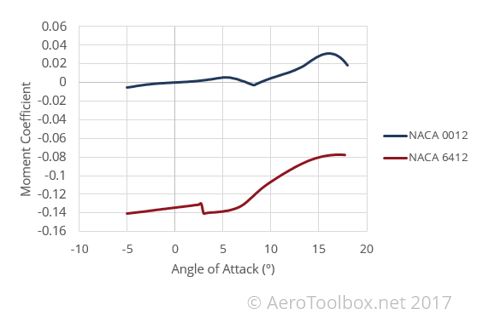
A plot of the quarter chord moment coefficient against angle of attack (shown below) shows how the airfoil responds to an increase in the angle of attack. A negative moment coefficient indicates a nose-down moment which will reduce the angle of attack of the aircraft in the absence of a control input. This is a desirable situation as this indicates that the aircraft will tend to resort to a condition in the linear lift region (stable) rather than the stall or post stall region (unstable). The aircraft static stability is a function not only of the geometry of the wing but the aircraft as a whole.
The trick when designing and specifying an airfoil profile for an aircraft is to try and ensure that the operating lift coefficient (usually the lift coefficient at cruise) corresponds to an angle of attack where the drag is at a minimum. This will produce an aircraft with an optimized lift-to-drag ratio which is the minimum drag configuration. However, this is only one design case to consider and often constraints such as a take-off distance requirement or maneuverability considerations result in a configuration that may be close to but not equal to the minimum drag case.
Wing design is a complex discipline and consists of optimizing the planform area and aspect ratio, designing for supersonic considerations (if applicable) and understanding the role that airfoil selection plays in the overall performance of the wing.
Thanks for reading this introduction to aerodynamic coefficients. If you enjoyed reading this please get the word out and share this post on your favorite social network!